Probabilistic forecast reconciliation
Daniele Girolimetto
Source:vignettes/articles/FoReco_prob.Rmd
FoReco_prob.RmdProbabilistic forecast reconciliation is a statistical procedure for
generating coherent and accurate forecasts across multiple time series.
FoReco is an R package that provides an implementation of
this technique, using the methods proposed by Panagiotelis et al. (2022)
and Girolimetto et al. (2023). The package is flexible and can be used
to perform reconciliation on cross-sectional, temporal, and
cross-temporal data. In particular we can calculate both point and
probabilistic forecasts, and allows for the specification of other
constraints (like non-negativity issues) to ensure that the forecasts
are consistent with each other. In this vignette, we will walk through
the basics of using FoReco for probabilistic forecast
reconciliation.
To get started, we need to load the necessary libraries and set a sample size for the probabilistic forecasts sample:
library(forecast) # the data and the forecasting function
library(MASS)     # simulate from a multivariate normal distribution
library(FoReco)   # bootstrap and reconciliation phase
B <- 1000         # Sample size for the probabilistic forecasts sample
Cross-sectional framework
Let’s take a look at how FoReco can be used for
cross-sectional reconciliation. In this scenario, we use the UKLungDeaths
dataset containing the monthly deaths from bronchitis, emphysema, and
asthma in the UK from 1974 to 1979 for both sexes
(Total), males (Male) and females
(Female). We want to generate coherent forecasts for
these variables, such that \(Total = Male +
Female\) at any time.

We start by arranging the data frame of deaths, the aggregation
matrix, and the constraint matrix. Then, we generate the base forecasts
with ETS model using the functions ets()
and forecast()
from the package forecast.
# Cross-sectional setup
tdeaths <- mdeaths + fdeaths
agg_mat <- t(c(1,1))
cons_cs <- cbind(1,-agg_mat)
lungDeaths <- cbind(tdeaths, mdeaths, fdeaths)

fit <- apply(lungDeaths, 2, function(x) ets(ts(x, frequency = frequency(lungDeaths))))
forecast_obj <- lapply(fit, forecast, h=12)      # forecast object
base <- sapply(forecast_obj, function(x) x$mean) # base mean (point forecasts)
res <- sapply(fit, residuals, type='response')   # in-sample residuals (one-step)
We know that a sample from the reconciled distribution can be obtained by reconciling each member of a sample from the incoherent distribution (Panagiotelis et al., 2022). This finding enables us to distinguish the process of generating the base forecast samples from the reconciliation phase. To generate an incoherent sample, we can use a non-parametric (such as the joint block bootstrap) or a parametric approach (by assuming gaussianity).
Bootstrap approach
We can implement the block bootstrap method proposed by Panagiotelis
et al. (2022) using the boot_cs() function. This function
requires three inputs: the fit parameter, which is a
list of models (e.g., the three ETS models used to forecast); the
boot_size parameter, which specifies the number of
bootstrap replications; h, which denotes the block
size, typically equivalent to the forecast horizon. It is important to
note that the models used have the simulate()
function available and implemented similarly to the package forecast
(Hyndman et al. 2023), with the following mandatory parameters:
object, innov,
future, and nsim. The outputs of the
function are the seed used to sample the errors, and a 3-d array (\(\mathrm{boot\_size} \times n \times h\)),
which can be reconciled using the htsrec() function.
# Base forecasts' sample:
# we simulate from the base models by sampling errors
# while keeping the cross-sectional dimension fixed.
base_csjb <- boot_cs(fit, B, 12)$sample
norm(apply(base_csjb, 3, function(x) x%*%t(cons_cs))) # Check the coherency for all the samples
#> [1] 120442.1

# Reconciled forecasts' sample:
# we reconcile each member of a sample from the incoherent distribution.
reco_csjb <- apply(base_csjb, 3, htsrec, C = agg_mat, res = res,
                   comb = "shr", keep = "recf", simplify = FALSE)
reco_csjb <- simplify2array(reco_csjb)
rownames(reco_csjb) <- NULL
norm(apply(reco_csjb, 3, function(x) x%*%t(cons_cs))) # Check the coherency
#> [1] 1.21986e-10
Gaussian approach
To obtain the base forecasts assuming Gaussianity (Panagiotelis et
al. 2022), we can use packages to simulate from a multivariate normal
distribution such as MASS
(Venables and Ripley 2002). We can then apply the htsrec()
function to obtain the reconciled sample. When dealing with multiple
forecast horizons, it is recommended to utilize multi-step residuals
instead of one-step residuals (see Girolimetto et al. 2023).
# Multi-step residuals
hres <- lapply(1:12, function(h)
  sapply(fit, residuals, type='response', h = h))
# List of H=12 covariance matrix (one for each forecast horizon)
cov_shr <- lapply(hres, function(r) shrink_estim(r)$scov)

# Base forecasts' sample:
# we simulate from a multivariate normal distribution.
base_csg <- lapply(1:12, function(h) MASS::mvrnorm(n = B, mu = base[h, ], Sigma = cov_shr[[h]]))
base_csg <- simplify2array(base_csg)
sum(abs(apply(base_csg, 3, function(x) x%*%t(cons_cs)))) # Check the coherency
#> [1] 1219109

# Reconciled forecasts' sample:
# we reconcile each member of the base forecasts' sample.
reco_csg <- apply(base_csg, 3, htsrec, C = agg_mat, res = res, comb = "shr", keep = "recf", simplify = FALSE)
reco_csg <- simplify2array(reco_csg)
rownames(reco_csg) <- NULL
sum(abs(apply(reco_csg, 3, function(x) x%*%t(cons_cs)))) # Check the coherency
#> [1] 1.05031e-09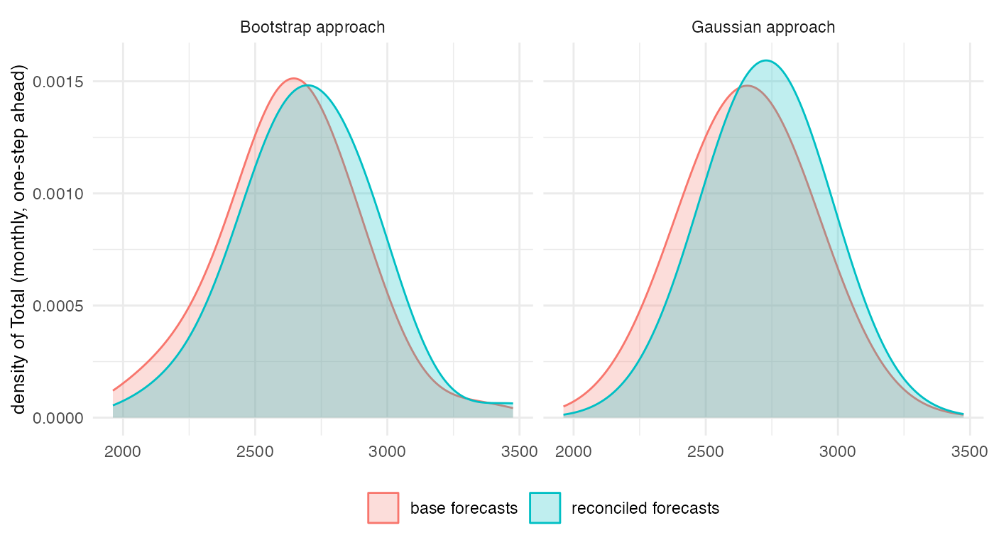
Temporal framework
In the temporal framework, we reconcile base forecasts across different time frequencies (e.g., monthly, quarterly, and annual data) for a single time series. For example, suppose we want to generate reconciled monthly, quarterly, and annual forecasts for the total number of deaths due to bronchitis, emphysema, and asthma in the UK. According to Girolimetto et al. (2023), we can use the same approach as in the cross-sectional framework, but we need to account for the different time frequencies.
In the bootstrap approach, we can use the boot_te()
function, which generates a bootstrap sample for time-series forecasts
while keeping a temporal structure. The function requires the same
inputs as the equivalent cross-sectional boot_cs()
function, with an additional parameter m that indicates
the maximum order of temporal aggregation. The length of the block
bootstrap is determined by both m and
h, where h refers to the forecast
horizons for the most temporally aggregated series.
In the Gaussian approach, we assume that all the base forecasts
follow a multivariate normal distribution, and we calculate the
covariance matrix of the base forecasts using multi-step residuals
organized in matrix form through the residuals_matrix()
function.
To reconcile each sample we use the optimal temporal reconclition
function, thfrec().
# Temporal setup
y <- tdeaths
m <- 12
kset <- c(12, 3, 1) # factors subset of m = 12
                    # (only monthly, quarterly and annual data are considered)
kset <- setNames(kset, paste0("k", kset))
cons_te <- thf_tools(m = kset)$Zt

temp_y <- lapply(kset, agg_ts, x = y)                         # Aggregated time series list
fit <- lapply(temp_y, function(x) ets(ts(x, frequency = frequency(x))))
forecast_obj <- lapply(fit, function(tsfit)
  forecast(tsfit, h=frequency(tsfit$x)))                      # forecast object
base <- sapply(forecast_obj, function(x) x$mean)              # base mean
res <- Reduce("c", sapply(fit, residuals, type='response'))   # in-sample residuals (one-step)
Bootstrap approach
# Base forecasts' sample:
# we simulate from the base models by sampling errors
# while keeping the temporal dimension fixed.
base_tejb <- boot_te(fit, B, m = kset)$sample

# Reconciled forecasts' sample:
# we reconcile each member of the base forecasts' sample.
reco_tejb <- t(apply(base_tejb, 1, function(boot_base){
  thfrec(boot_base, m = kset, res = res, comb = "wlsv", keep = "recf")}))
Gaussian approach
# Multi-step residuals
hres <- lapply(fit, function(mod)
  lapply(1:frequency(mod$x), function(h)
    residuals(mod, type='response', h = h)))
hres <- Reduce("c", lapply(hres, arrange_hres))
# Re-arrenge multi-step residuals in a matrix form
mres <- residuals_matrix(hres, m = kset)

# Base forecasts' sample:
# we simulate from a multivariate normal distribution.
base_teg <- MASS::mvrnorm(n = B, mu = unlist(base), Sigma = shrink_estim(mres)$scov)

# Reconciled forecasts' sample:
# we reconcile each member of the base forecasts' sample.
reco_teg <- t(apply(base_teg, 1, thfrec, m = kset, comb = "wlsv", res = res, keep = "recf"))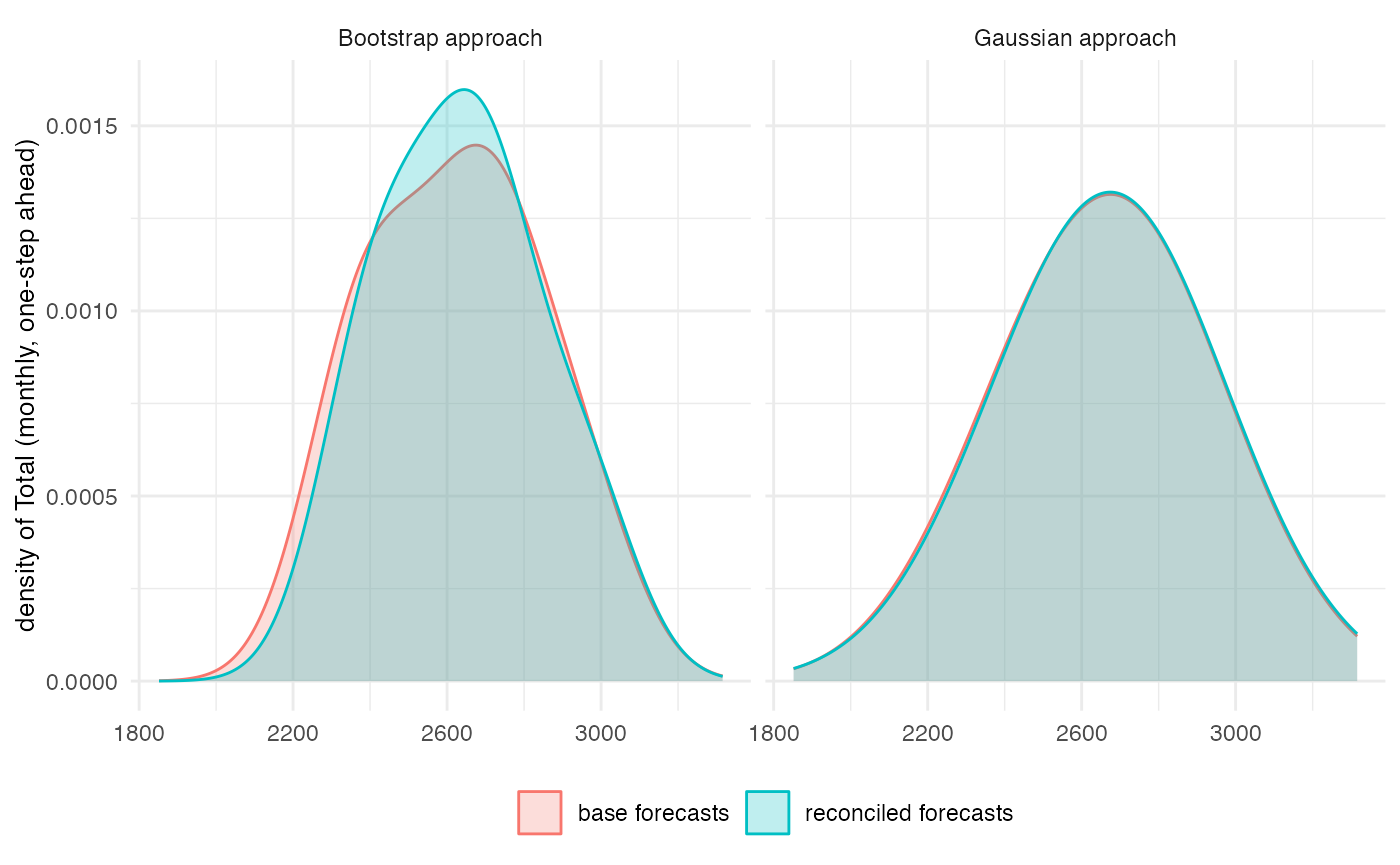
Cross-temporal framework
Finally, we obtain probabilistic reconciled forecasts in the
cross-temporal framework. We use the boot_ct() function
with almost the same input as boot_te() to implement the
bootstrap approach. The fit parameter in this case has
to consider the model for all the series at different frequency.
For the Gaussian approach, we can use the arrange_hres()
and residuals_matrix() functions to arrange residuals for
the covariance matrix of the base forecasts.
Finally, we can reconcile the base forecasts samples with the optimal
cross-temporal reconciliation octrec() (or we can use other
heuristic alternatives, e.g. iterec()).
# Cross-temporal setup
ctlungDeaths <- lapply(kset, agg_ts, x = lungDeaths) # Aggregated multivariate time series list

fit <- lapply(ctlungDeaths, function(tsk)
  apply(tsk, 2, function(x) ets(ts(x, frequency = frequency(tsk)))))
forecast_obj <- lapply(fit, function(fitk)           # forecast object
  lapply(fitk, function(tsfit)
    forecast(tsfit, h=frequency(tsfit$x))))
base <- sapply(forecast_obj, function(fmodk)     # base mean
  sapply(fmodk, function(x) x$mean))
res <- Reduce("rbind", sapply(fit, function(fitk)    # in-sample residuals (one-step)
  sapply(fitk, residuals, type='response')))
Bootstrap approach
# Base forecasts' sample:
# we simulate from the base models by sampling errors
# while keeping the cross-sectional and temporal dimensions fixed.
base_ctjb <- boot_ct(fit, B, m = kset)$sample

# Reconciled forecasts' sample:
# we reconcile each member of the base forecasts' sample.
reco_ctjb <- lapply(base_ctjb, function(boot_base){
  octrec(t(boot_base), m = kset, C = agg_mat, res = t(res), comb = "bdshr", keep = "recf")})
reco_ctjb <- lapply(reco_ctjb, function(x) `rownames<-`(t(x), NULL))
Gaussian approach
# Multi-step residuals
hres <- lapply(fit, function(fitk)    # in-sample residuals (one-step)
  lapply(1:frequency(fitk$tdeaths$x), function(h)
    sapply(fitk, residuals, type='response', h = h)))
hres <- t(Reduce("rbind", lapply(hres, arrange_hres)))
# Re-arrenge multi-step residuals in a matrix form
mres <- residuals_matrix(hres, m = kset)

# Base forecasts' sample:
# we simulate from a multivariate normal distribution.
base_ctg <- MASS::mvrnorm(n = B, mu = residuals_matrix(t(Reduce("rbind", base)), m = kset),
                          Sigma = cov(na.omit(mres)))
base_ctg <- apply(base_ctg, 1, function(x) matrix(x, ncol = 3), simplify = FALSE)

# Reconciled forecasts' sample:
# we reconcile each member of the base forecasts' sample.
reco_ctg <- lapply(base_ctg, function(boot_base){
  FoReco::octrec(t(boot_base), m = kset, C = agg_mat, res = t(res), comb = "bdshr",
         keep = "recf")})
reco_ctg <- lapply(reco_ctg, function(x) `rownames<-`(t(x), NULL))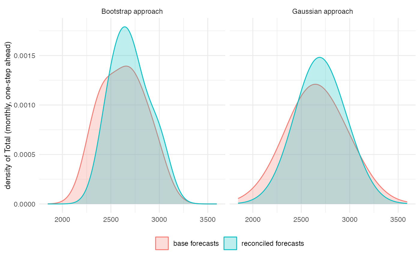
References
Girolimetto, D., Athanasopoulos, G., Di Fonzo, T., and Hyndman, R. J. (2023), Cross-temporal Probabilistic Forecast Reconciliation, https://doi.org/10.48550/arXiv.2303.17277 .
Hyndman R, Athanasopoulos G, Bergmeir C, Caceres G, Chhay L, O’Hara-Wild M, Petropoulos F, Razbash S, Wang E, Yasmeen F (2023). forecast: Forecasting functions for time series and linear models . R package version 8.20, https://pkg.robjhyndman.com/forecast/.
Panagiotelis, A., Gamakumara, P., Athanasopoulos, G. and Hyndman, R. J. (2023), Probabilistic forecast reconciliation: Properties, evaluation and score optimisation, European Journal of Operational Research 306(2), 693–706, https://doi.org/10.1016/j.ejor.2022.07.040 .