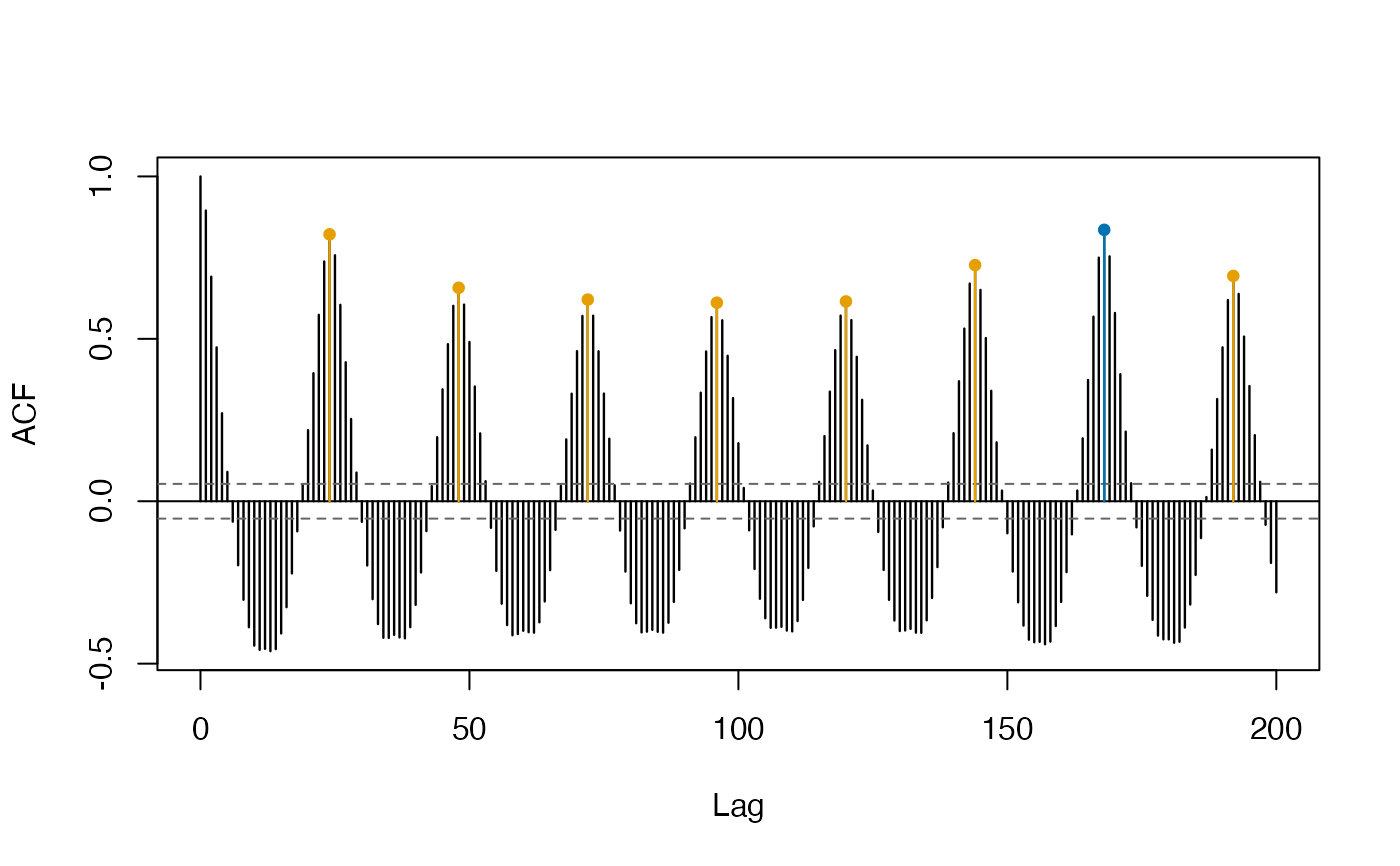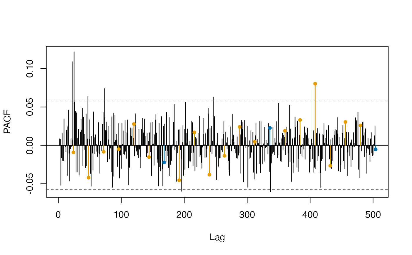
Sample autocorrelation (sacf) and partial autocorrelation (spacf) functions
that highlight the lags belonging to one or more seasonal cycles, so that the
seasonal structure of a multi-seasonal series is visible at a glance.
ggsacf() and ggspacf() are the ggplot2 equivalents.
Usage
sacf(
  x,
  season = NULL,
  lag.max = NULL,
  ci = 0.95,
  col = NULL,
  main = NULL,
  ylab = "ACF",
  plot = TRUE,
  ...
)

spacf(x, ..., ylab = "PACF")

ggsacf(
  x,
  season = NULL,
  lag.max = NULL,
  ci = 0.95,
  main = NULL,
  ylab = "ACF",
  ...
)

ggspacf(x, ..., ylab = "PACF")
Arguments
- x
A numeric vector, a
ts/mstsobject, or a fitted msarima model (in which case the model residuals are used).- season
Numeric vector of seasonal periods to highlight, of any length. If
NULL(default) the periods are taken from themsts/tsattributes ofx, or from the fitted model.- lag.max
Maximum lag. Defaults to
3 * max(season), or to the stats::acf default when no seasonal period is available.- ci
Coverage of the confidence bands, as a probability. Default
0.95.- col
Colours used for the seasonal lags, one per element of
season(recycled). Defaults to a colour-blind safe palette (Okabe and Ito, 2008), the same one used byggsacf()andggspacf().- main, ylab
Plot title and y-axis label.
- plot
If
TRUE(default) the correlogram is drawn.- ...
Further arguments passed to stats::acf, and from
spacf()andggspacf()tosacf()andggsacf().
Value
sacf() and spacf() invisibly return the stats::acf object, with
the seasonal periods in the "season" attribute and, for each lag, the index
of the period it belongs to in "season.group". ggsacf() and ggspacf()
return a ggplot object.
Details
Lags that are multiples of more than one period (lag 168 with
season = c(24, 168), say) are attributed to the longest matching period.
The series is treated as a plain numeric vector, so lags are always reported in
number of observations and not in units of time. Leading and trailing NAs,
such as those produced by differencing in msarima, are dropped
(stats::na.contiguous).
References
Okabe, M. and Ito, K. (2008). Color Universal Design (CUD): How to make figures and presentations that are friendly to colorblind people. https://jfly.uni-koeln.de/color/