
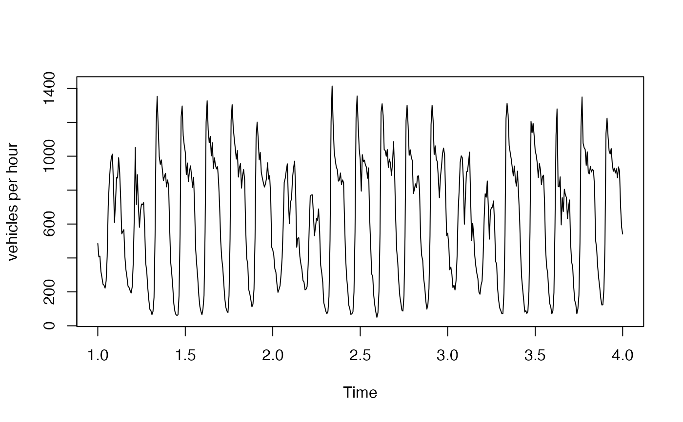
Number of vehicles per hour recorded by a single traffic sensor on the M-40, the outer ring road of Madrid, over the eight weeks from 3 February to 29 March 2024.
The series shows the two seasonal patterns that msarima is meant for:
a daily cycle of period 24, with the morning and evening commuting peaks, and a
weekly cycle of period 168, with markedly lower volumes at the weekend.
Format
An msts object of length 1344 (56 days, or eight complete weeks, of hourly
data) with seasonal periods 24 and 168. The first observation is midnight of
Saturday 3 February 2024 and the last is 11 p.m. of Friday 29 March 2024.
Source
Madrid City Council open data portal, https://datos.madrid.es.
Details
The raw measurements are half-hourly counts from sensor 3753, recorded between 1 February and 31 May 2024 and summed in pairs to obtain hourly volumes; the eight weeks kept here are the window studied by Grigoletto and Lisi (2026), who chose this sensor for having the fewest missing observations in the network. A few of the underlying half-hourly counts had been interpolated by the provider, so 3 of the hourly values are not whole numbers. There are no missing values and no gaps in the hourly grid.
The script that builds the object from the raw file is available at https://github.com/danigiro/msarima/blob/main/data-raw/MAD_m40.R.
References
Grigoletto, M. and Lisi, F. (2026). Portmanteau goodness-of-fit tests in the presence of simple, mixed, and multiple seasonal autocorrelation. arXiv. doi:10.48550/arXiv.2609.32381
Examples
# The daily and weekly cycles
plot(window(MAD_m40, end = 4), ylab = "vehicles per hour")
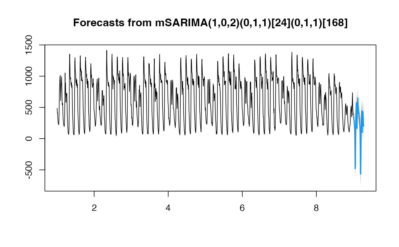
 # A multi-seasonal ARIMA with one daily and one weekly difference
# \donttest{
fit <- msarima(MAD_m40,
order = c(1, 0, 2),
seasonal = list(c(0, 1, 1), c(0, 1, 1)))
summary(fit)
#> Series: MAD_m40
#> mSARIMA(1,0,2)(0,1,1)[24](0,1,1)[168]
#>
#> Coefficients:
#> Estimate Std. Error z value Pr(>|z|)
#> AR(1) 0.88473 0.02473 35.770 <2e-16 ***
#> MA(1) -0.37373 0.04060 -9.204 <2e-16 ***
#> MA(2) -0.09059 0.03805 -2.381 0.0173 *
#> SMA(1,1) -0.56029 0.02700 -20.748 <2e-16 ***
#> SMA(2,1) -0.68362 0.02525 -27.072 <2e-16 ***
#> ---
#> Signif. codes: 0 ‘***’ 0.001 ‘**’ 0.01 ‘*’ 0.05 ‘.’ 0.1 ‘ ’ 1
#>
#> sigma^2 = 4009.7288 log likelihood = -5356.4828
#> AIC = 10724.9656 AICc = 10725.0390 BIC = 10755.2612
plot(forecast(fit, h = 48))
 # }